Contents of this chapter
-
II.1 Basic Operations
-
II.2 Schema Theorem and Theoretical Background
-
II.3 Solving a Problem: Genotype and Fitness
-
II.4 Models of Evolution
-
II.5 Advanced Operators
-
II.6 Non-Conventional Genotypes
-
II.7 Important Issues in the Implementation of a GA
-
II.8 Response to Selection
II.1 Basic Operations
The basic operations first performed by a GA are the generation and evaluation
of an initial population. Subsequently, a main loop of operations that
include selecting the best individuals, crossing them and applying mutation
on every locus (string position) is done. The solution is usually the best
string that is present in the final population.
The computational effort in a normal GA usually resides in the evaluation
of the initial and new strings. Normally the fitness function is complex:
a mathematical function with many parameters, a full neural network that
needs to inspect dozens of patterns for computing one single (float) fitness
value, the simulation of a given system that yields a figure of merit of
the string for this system, etc... Operators like selection, mutation,
crossover or replacement are of linear complexity and work at constant
rates for a given problem.
 A traditional GA works on binary strings of fixed length and applies fitness
proportionate selection, one point crossover and bit-flip mutation. The
initial population is generated by following an uniform random distribution,
that is, every position in every string contains one 0 or one 1 with the
same probability (0.5). The evolution model is represented by successive
generations of populations, i.e., a new population completely replaces
the old one. The algorithm stops when a predefined number of generations
have been reached. Finally the evaluation of any given string is made by
mapping the genotype to the phenotype by means of a binary-to-decimal operation
for every group of bits of the genotype representing one problem parameter.
II.2 Schema Theorem and Theoretical Background
The theoretical basis of genetic algorithms relies on the concept of schema
(pl. schemata). Schemata are templates that partially specify
a solution (more strictly, a solution in the genotype space). If genotypes
are strings built using symbols from an alphabet A, schemata are
strings whose symbols belong to A U {*}. This extra-symbol must
be interpreted as a wildcard, being loci occupied by it called undefined.
A chromosome is said to match a schema if they agree in the defined positions.
For example:
The string 10011010 matches the schemata
1******* and **011***
among others, but does not match *1*11***
because they differ in the second gene (the first defined gene in the schema).
A schema can be viewed as a hyperplane in a  -dimensional
space representing a set of solutions with common properties. Obviously,
the number of solutions that match a schema H depend on the number
of defined positions in it (its order, represented o(H)).
Another related concept is the defining-length (represented
  (H))
of a schema, defined as the distance between the first and the last defined
positions in it. See Table 1 for examples.
|
Schema H
|
o(H)
|
 (H) (H)
|
|
1*******
|
1
|
0
|
|
**011***
|
3
|
2
|
|
*1*11***
|
3
|
3
|
Table 1. Examples of schemata.
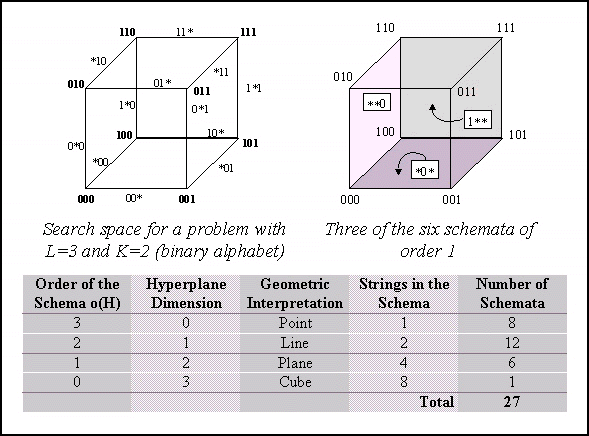
Figure 2. The Concept of Schema.
The GA works by allocating strings to best schemata exponentially through
successive generations, being the selection mechanism the main responsible
for this behavior. On the other hand the crossover operator is encharged
for exploring new combinations of the present schemata in order to get
fittest individuals. Finally the purpose of the mutation operator is to
introduce fresh genotypic material in the population (it is specially important
as generations proceed).
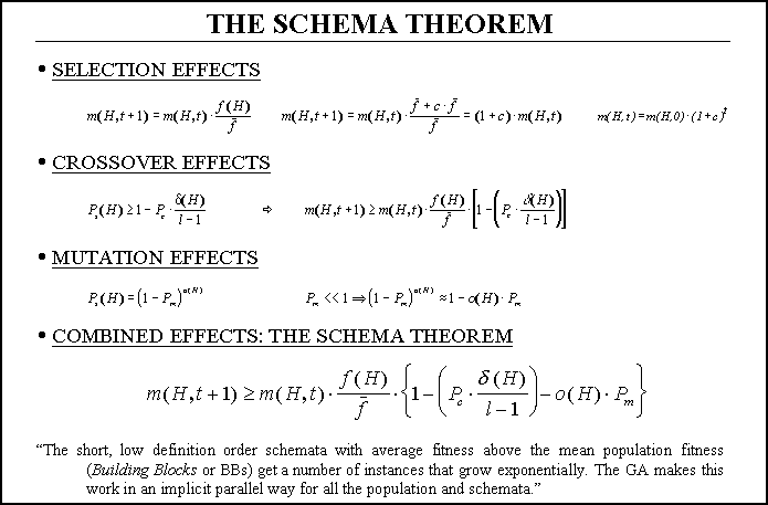
Figure 3. Derivation of The Schema Theorem.
All this behavior is analytically described by the so-called schema
theorem, where P's are the probabilities of crossover and mutation
and m(H,t) is the number of instances (strings) the schema H
has in the generation number t.

Figure 4. The Schema Theorem.
II.3 Solving a Problem: Genotype and Fitness
In order to apply a GA to a given problem the first decisions one has to
make are concerning the kind of genotype the problem needs. That means
that you must decide how the parameters of your problem maps into a binary
string (if a binary string is to be used at all). This implies that you
must choice the number of bits per parameter, the range of the decoded
binary-to-decimal parameter, if the strings have constant or changing lengths
during the GA operations, etc...
In traditional applications the strings use a binary alphabet and their
length is constant during all the evolution process. Also all the parameters
decode to the same range of values and are allocated the same number of
bits for the genes in the string.
In most recent applications this situation is changing in a very important
way. More and more complex applications need dynamic length strings or
else a different non-binary alphabet. Typically integer or float genes
are using in many domains as neural networks training, function optimization
with a large number of variables, reordering problems as the Traveling
Salesperson Problem, etc...
The traditional concept of a schema advises the utilization of binary
genes because the number of schemata sampled per string is maximized. But
a new interpretation of the schema concept has arrived to explain why many
people have found very useful using other non-binary genes. This new interpretation
(Antonisse, 1989) considers
benefitial the utilization of higher cardinality alphabets due to their
higher expression power (as many traditional AI paradigms consider). It
is based on the consideration of the wildcard symbol (*) as an instantiation
character for different sets of symbols and not the traditional wildcard
symbol. To be precise, * is reinterpreted as a family of symbols *x,
where x can be any subset of symbols of the alphabet. For binary
strings these two interpretations are the same but for higher cardinality
alphabets they are not.
Regarding genotypes, many other developments have pushed forward the
utilization of non-string representations such as trees of symbols (e.g.
Genetic Programming (Koza, 1992))
that are much more appropriate for a large number of applications. Also
extending every allele of the string along with the position (locus) it
occupies in the string is interesting because we can freely mix the genes
of the same string in order to get together the building blocks automatically
during evolution. This is very interesting when we do not know which are
the building blocks of our problem and want the GA to discover them. By
associating the locus to every gene value we can reorder the string in
the correct way before evaluating the string. These mechanism are common
to the so-called messy GAs (Goldberg,
Deb, Korb, 1991).
Here we arrive to the problem of decoding (called expression)
the genotype to yield the phenotype, that is, the string of problem parameters.
This is necessary since we need to evaluate the string in order to assign
it a fitness value. Thus we use the phenotype as the input to the fitness
function and get back a fitness value that helps the algorithm to relatively
rank the strings in the population pool.
The construction of an appropriate fitness function is very important
for the correct work of the GA. This function represents the problem environment,
that is, it decides who much well the string solves the problem. Many problems
arise when the fitness function has to be constructed:
Regarding dynamic fitness functions a genotype of diploid genes can be
used in which every value is determined by some relationship among two
alleles encoded in the same string. The extension to K-ploid strings
is straightforward. A dominance operator needs to be defined in
order to get a single gene (parameter) value from the K alleles
that determine it.
As the evolution proceeds the fitness values assigned by the fitness
function to the strings are very similar since the strings we are evaluating
are also very similar. There exist some different scaling operators
that help in separating the fitness values in order to improve the work
of the selection mechanism. The most common ones are (Michalewicz,
1992):
-
Linear Scaling: f'=af+b
-
Sigma Truncation: f'=max[0, f-(f*-c
 )],
where f* (resp.
  )
is the mean fitness value (resp. standard deviation) in the population.
-
Power Scaling: f'=(f)^k
Also when very different strings get the same fitness values an important
problem arises in that crossing them yield very bad individuals (called
lethals) unable of further improvements. Sharing methods
(Goldberg, 1989) help to allow
the concurrent existence of very different solutions in the same genetic
population. Also parallel models help in overcoming this problem.
Sometimes is very interesting to rank the population according to the
fitness values of the strings and then to apply a reproductive plan that
uses the rank position of the strings instead of the fitness values. This
is good for ill-designed fitness function or when very similar fitness
values are expected. This mechanism is called ranking (Whitley,
1989), and keeps a constant selection pressure on the population.
II.4 Models of Evolution
In traditional GAs the basic evolution step is a generation of individuals.
That means that the atomic advance step of the GA is one generation. There
exists another interesting alternative called Steady-State GAs in
which the atomic step is the computation of one single new individual.
In these algorithms after generating the initial population, the GA proceeds
in steps that consist of selecting two parents, crossing them to get one
(or two) single individual and mutating the resulting offspring. The new
string is inserted back in the population and one of the pre-existing strings
(a random string or the worst present string) leave the pool (normally
if the new string is worst than the actual worst it is not inserted at
all).
This one-at-a-time reproduction was initially introduced to overcome
problems in the training of neural networks and was extended from there
to the rest of present applications. It represents an interesting equilibrium
between the exploration and exploitation edges of a GA, because the GA
maintains a pool of strings (exploration, schemata, etc...) and at the
same time it performs some kind of hill-climbing since the population is
only pushed torward better solutions. Elitism and ranking are very common
to steady-state GAs.
Finally there exists an intermediate model of evolution for a sequential
GA in which a percentage of the full population is selected for the application
of genetic operations. This percentage is called the GAP and it
represents the generalization of any evolution model since it includes
the two apposite approaches (generations versus one-at-a-time) and any
other intermediate model.
Many other models of evolution exist in the field of parallel GAs depending
on their granularity, homogeneity, etc... but we will discuss them in a
following chapter.
II.5 Advanced Operations
Besides the traditional operations, a GA can incorporate new techniques
at different levels. One of the most used innovations is to define new
genetic operators improving in some way the behaviour of the general one-point
crossover or bit-flip mutation for certain problems. Normally these new
operators are the result of a theoretical study of GAs or else they are
new versions of traditional operators that incorporate problem-dependent
knowledge.
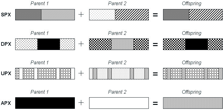
Figure 5. Some Examples of New Crossover Techniques:
Single-Point, Double-Point, Uniform and Arithmetic Crossover Operators.
Also advanced genotypes can be used instead of the traditional binary encoding.
Finally new schemes of evolution (steady-state, parallelism, ...) or foreign
operators (hillclimbing operators, existing algorithms, ...) can be added
to the GA skeleton, being applied with a given probability of success as
the next generation is being created from the previous one.
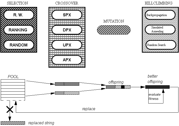
Figure 6. A Steady-State GA Architecture with Different
Operators.
II.6 Non-Conventional Genotypes
As mentioned before, genetic algorithms have traditionally used a pure
binary genotype in which every parameter of the problem is encoded in binary
by using a given number of bits. The number of bits for every gene (parameter)
and the decimal range in which they decode are usually the same but nothing
precludes the utilization of a different number of bits or range for every
gene.
In order to avoid the so-called hamming cliffs the gray code
is sometimes used when decoding a binary string. With this code any two
adjacent decimal values are encoded with binary numbers that only differ
in one bit. This helps the GA to make a gracefully approach to an optimum
and normally reduces the complexity of the resulting search.
Nevertheless, the plethora of applications to which GAs have been faced
have motivated the design of many different genotypes. This means that
the string can be constructed over an integer or real alphabet, for example.
Integer alphabets have interesting properties for reordering problems such
as the Traveling Salesperson Problem and others. On the other hand floating-point
genes are very useful for numeric optimization (for example for neural
network training). These higher cardinality alphabets enhance the search
by reducing the number of ill-constructed strings resulting from the application
of crossover or mutation. Also, when a very large number of parameters
has to be optimized, it is helpful to rely on shorter strings (also because
populations and the number of steps are smaller).
If the genotype can be expressed as a string, we need to decide for
any given application if the genome length is going to be kept constant
or allowed to change. Also, it is an interesting decision to use diploid
individuals in dynamic environments (i.e., environments in which the fitness
function changes as the search proceeds). In a diploid individual two -homologous-
chromosomes describe the same set of parameters. When decoding the string
some kind of dominance operator need to be used in order to decide
the value of the problem parameter (gene).
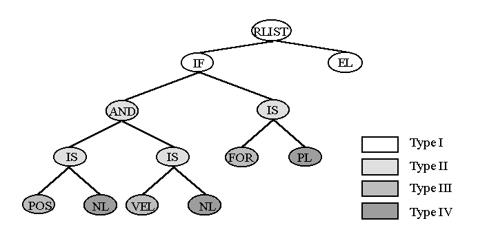
In many recent applications more sophisticated genotypes are appearing:
II.7 Important Issues in the Implementation of
a GA
It follows an initial summary of issues relating the implementation of
a sequential GA:
II.8 Response to Selection
In this section we summarize of the theory presented in Mühlenbein
and Schlierkamp-Voosen (1995). Let  be
the average fitness of the population at generation t. The response
to selection is defined as
 .
.
The amount of selection is measured by the selection differential
 ,
,
where  is
the average fitness of the selected parents. The equation for the response
to selection relates R and S:
 .
.
The value b(t) is called the realized heritability.
For many fitness functions and selection schemes, the selection differential
can be expressed as a function of the standard deviation  of
the fitness of the population. For truncation selection (selecting
the T·N best individuals) and for normally distributed fitness,
the selection differential is proportional to the standard deviation:
 .
.
The vaule I is called the selection intensisty.
For arbitrary distributions one can show the following estimate:
 .
.
For normally distributed fitness the famous equation for the
response to selection is obtained:
 .
.
The above equation is valid for a large range of distributions,
not just for a normal distribution. The response depends on the selection
intensity, th realized heritability, and the standard deviation of the
fitness distribution. In order to use the above equation for prediction,
one has to estimate b(t). The equation also gives a design
goal for genetic operators -- to maximize the product of heritability
and standard deviation. In other words, if two recombination operators
have the same heritability, the operator creating an offspring population
with larger standard deviation is to be preferred.
The equation defines also a design goal for a selection method
-- to maximize the product of selection intensity and standard deviation.
In simpler terms, if two selection methods have the same selection intensity,
the method giving the higher standard deviation of the selected parents
is to be preferred. For proportionate selection as used by the simple genetic
algorithm (Goldberg, 1989) it
was shown by Mühlenbein and Schlierkamp-Voosen (1993) that
 .
.
The equation shows that the selection intensity of proportionate
selection goes to zero for t  inf,
whereas truncation selection has a constant selection intensity. Proportionate
selection selects too weak in the final stages of the search.
This page was last updated on 06-Apr-98


 .
.