RND Problem Description

The radio coverage problem amounts to covering an area with a set of transmitters. The part of an area that is covered by a transmitter is called a cell. A cell is usually not connex. In the following we will assume that the cells and the area considered are discretized, that is, they can be described as a finite collection of geographical locations (taken from a geo-referenced grid, for example). The computation of cells may be based on sophisticated wave propagation models, on measurements, or on draft estimations. In any case, we assume that cells can be computed and returned by
an ad hoc function. 

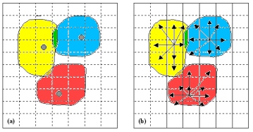
    Let us consider the set L of all potentially covered locations and the set M of all potential transmitter locations. Let G be the graph, (M U L, E), where E is a set of edges such that each transmitter location is linked to the locations it covers and let be the vector x a solution to the problem where x belongs to {0,1}, and i is in [1,149]  indicates whether a transmitter is being used or not. As the geographical area needs to be discretized, the potentially covered locations are taken from a grid, as shown in the Figure 1.

Figure1. (left) Three potentially transmitter locations and their associated covered cells on a grid, and (right) graph representing covered locations.

    Searching for the minimum subset of transmitters that covers a maximum surface of an area comes to searching for a subset M' contained in M such that |M'| is minimum and such that |Neighbors (M',E)| is maximum, where 

   (Eq. 1)

    The problem we consider recalls the unicost set covering problem (USCP) that is known to be NP-Hard. The radio
coverage problem differs, however, from the USCP in that the goal is to select a subset of transmitters that ensures a
good coverage of the area and not to ensure a total coverage. The difficulty of our problem arises from the fact that the goal is twofold, no part being secondary. If minimizing was the primary goal, the solution would be trivial: M' equal to the empty set. If maximizing the number of covered locations was the primary goal, then problem would be the USCP. An objective function f(x) to combine the two goals is:

  (Eq. 2)

where

  (Eq. 3)

the parameter alpha can be tuned to favor the cover rate with respect to the number of transmitters. We will use alpha=2 and a 287 * 287 point grid representing an open-air flat area. Also, 49 primary transmitter locations are distributed regularly in this area in order to form a 7 * 7 grid structure, and each transmitter has an associated 41 *  41
point cell.

    Consequently, the obtained coverage would be total if the algorithm happens to assign one transmitter to these locations. A hundred complementary transmitters locations were then randomly selected, associated to 41 \times 41 point cells (fewer when clipped by the border of the area), and shuffled with the 49 primary ones. By construction, the best solution is the one that covers 100\% of the area with the 49 primary transmitters (giving a fitness value of 204.08). See in Figure 2  the graphical representation of a partial (left) and optimal (right) solution for the RND problem.

Figure 2. Graphical representation of a partial solution covering 85.8\% of the whole area, and (right) a graphical representation of an optimal solution.

    Designing a fitness function is one of the most important steps in applying an evolutionary algorithm to a new problem. The kind of representation being used in the algorithm influences its use inside the fitness function. In this section, we will address the definition of the fitness function and the interpretation of the GA strings that hopefully will guide the algorithms towards the problem regions where the solution reside.

In our representation, every potential transmitter location is assigned a bit in the binary string manipulated in the algorithm. A 1 in a given string position means that the associated transmitter will be used in the placement, i.e. more points are potentially covered in the grid and one more transmitter needs to be considered in all the computations inside the fitness function.

    The fitness function accounts for all problem knowledge details in that it scan the binary string provided by the algorithm, therefore computing the covered area as well as other statistical measures that could be needed to assess the quality of the evaluated individual as a tentative solution to the problem. In our case we will investigate the relative performances of two evaluation functions.

    The first one (equation 2) is a fitness function that directly follows the problem definition given in this page, thus computing the ratio between the covered versus the total area in the problem (the grid). We maximize the covered area and, at the same time, we penalize solutions having a large number of transmitters.

    This first evaluation function works out a considerably high time before computing a solution. Therefore, we test a second fitness function that could directly account for some features that an optimal solution should have, thus hopefully reducing the number of sampled points. In particular, we know that an optimal solution for this problem should not leave any point in the grid without coverage, and this means that the mean number of transmitters covering a single
point should be 1.0. This is computed in a penalty term P_m explained in equation 4. 

       (Eq. 4)

    But it is not enough to have a mean number of transmitters of 1.0 over each point in the target area. In addition, it should hold for the standard deviation to have a value of 0.0, since in this way we could assure that each point is covered by one and only one transmitter in the solution. See this second penalty term P_v in equation 5.

        (Eq. 5)

    We have called these two terms penalty values since we plan to penalize the first evaluation function with they two in order to try the algorithm to have a better guide along the search space. See in equation 6 the resulting evaluation
function intended to be maximized by the algorithms.

        (Eq. 6)

    Therefore, we are going to compare the results by using these two evaluation functions throughout our tests. It is expected for the second function to be harder to compute, since we need to calculate more statistical info inside the problem simulator embedded in the fitness function; on the contrary, we expect it to find out a solution in a smaller search time (despite the overload of computing additional statistics in this function). Take a look to Table 1 to see the pseudo-codes of these functions in a C-like style. With the help of two functions computing the covered area and the number of used transmitters contained in a binary-encoded solution x, we can freely compute the rest of needed values.

    See in Table 2 the numeric ranges of the fitness values returned by each of the maximized functions. We computed the constants a_i, b_i to have the same range in these functions to make more understandable the tests.

Table 2.Numeric ranges for the result of every fitness function.

Home | Introduction on EAs | xxGA | Problems | Links | Articles DB