
RND Problem Result
In this section we present the results of performing an assorted set of tests by using sequential and parallel GAs to solve the RND problem (both evaluation functions are considered throughout).
First, we will analyze the number of evaluations and time needed by either configuration. Let us begin considering a sequential implementation of a steady state GA with a single population of 512 individuals, using a normal parameterization, namely roulette wheel selection of each parent, two-point crossover with probability 1.0, bit-flip mutation with probability 1/strlen and replacement always of the worst string. Then we will analyze the results of a parallel steady state GA having 8 islands, each one with 64 individuals performing in parallel the mentioned basic evolutionary step, with an added migration operation. The migration will occur in a unidirectional ring manner sending one single randomly chosen individual to the neighbor sub-population. The target population incorporates this individual only if it is better than its presently worst solution. The migration step is performed every 2048 iterations in every island in an asynchronous model, since it is expected to be more efficient than a synchronous execution over the pool of available processors. We will run this algorithm both in one single CPU (i.e., concurrently) and on 8 processors. Each processor is an Ultra Sparc 1 CPU at 143 Mhz with 64Mb RAM. See a summary of the conditions for experimentation in table below.
| Population Size | 512 |
| Selection | Roulette Wheel |
| Crossover | tpx 1.0 |
| Mutation | Probability 0.00671 |
| Replacement | Least fitted |
| Number of islands | 8 |
| Migration policy for selection | Random selection |
| Migration policy for replacement | Replace if better |
| Migration gap | 2048 |
| Number of migrants | 1 |
| Synchronization | Asynchronous mode |
Table 1. Parameters of the algorithms being used
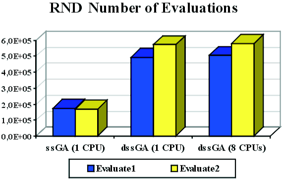
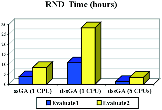
In table 2 we give the numeric values of measuring the number of evaluations and the running time for both algorithms, the ssGA and the distributed ssGA with 8 islands (this last running in 1 processor and also in 8 processors).
|
Evaluate1
|
Evaluate2
|
|||
|
# evaluations
|
time (hours)
|
# evaluations
|
time (hours)
|
|
|
dssGA (8 CPUs)
|
505624
|
1.38
|
579922
|
3.53
|
|
dssGA (1 CPU)
|
491493
|
10.87
|
573175
|
28.41
|
|
ssGA
|
173013
|
3.86
|
169016
|
8.49
|
Table 2. Number of evaluations (left) and time (right) with ssGA and dssGA for Evaluate1 and Evaluate2.
To asses the statistical significance of the results we performed
30 independent runs and then computed the Student t-test analysis so that we
could be able to distinguish meaningful differences in the average values. The
significance p-value is assumed to be 0.05, in order to indicate a 95\%
confidence level in the numeric differences in the means. See in Tables 3 and
4 these statistical assessment of the results for the number of evaluations
and the execution time, respectively.
|
t-test
|
dssGA(8 CPUs)
|
dssGA(1 CPU)
|
ssGA
|
dssGA(8 CPUs)
|
dssGA(1 CPU)
|
ssGA
|
|
dssGA(8 CPUs)
|
-
|
0.7380
|
6.02·10-14
|
-
|
0.8711
|
9.36·10-14
|
|
dssGA(1 CPU)
|
0.7380
|
-
|
2.86·10-11
|
0.8711
|
-
|
< 2.2·10-16
|
|
ssGA
|
6.02·10-14
|
2.86·10-11
|
-
|
9.36·10-14
|
< 2.2·10-16
|
-
|
|
t-test
|
dssGA(8 CPUs)
|
dssGA(1 CPU)
|
ssGA
|
dssGA(8 CPUs)
|
dssGA(1 CPU)
|
ssGA
|
|
dssGA(8 CPUs)
|
-
|
3.48·10-14
|
4.55·10-09
|
-
|
< 2.2·10-16
|
3.63·10-12
|
|
dssGA(1 CPU)
|
3.48·10-14
|
-
|
2.32·10-11
|
< 2.2·10-16
|
-
|
< 2.2·10-16
|
|
ssGA
|
4.55·10-09
|
2.32·10-11
|
-
|
3.63·10-12
|
< 2.2·10-16
|
-
|
If we interpret the results in Table
2 we can notice several facts. Firstly, for Evaluate1, it is clear that the
sequential ssGA is the best algorithm numerically, since it samples almost 3
times less number of points in the search space before locating an optimal solution.
As to the search time, the best algorithm is thedssGA heuristic on 8 processors,
since it performs very quickly (1.38 hours) in comparison with the ssGA (3.86
hours), and the dssGA on a single processor (10.87 hours). This comes as no
surprise since numerically, ssGA was better, although dssGA on 8 processors
makes computations much faster. Since it is not fair to compute speedup against
a panmictic ssGA we compare the same algorithm, both in sequential and
parallel (dssGA on 8 versus 1 processors), with the stopping criterion of getting
a solution of the same quality. We then find out that speedup is 7.87, i.e.
near linear speedup, which is very satisfactory.
For the second fitness function (see Table 2 again) we can
notice that the results are much the same: ssGA is numerically advantageous
with respect both execution scenarios of dssGA. These two last algorithms seem
again to provide the same average number of evaluations (differences are not
significant, since the t-test offers a value clearly larger than 0.05, the significance
level). Again, the execution time relationship is just like with the first evaluation
function (in fact, speedup is perfect, even slightly superlinear: 8.04).
Therefore, the conclusions are that, numerically speaking,
ssGA is the best algorithm for any of the evaluation functions. It can also
be concluded that the second evaluation function do not reduce the number of
sampled points before getting a solution, despite we expected it. In addition,
the execution time of all the algorithms is clearly enlarged when using Evaluate2.
See a graphical interpretation of the results in Figure 1 and 2, were we plot
the average number of
evaluations and execution time for ssGA and for the serial and parallel versions
of dssGA.
|
|
|
Figure 1. Number of evaluations (left) and time (right) needed by (d)ssGA to solve RND.
| Home | Introduction on EAs | xxGA | Problems | Links | Articles DB |