To run the metaheuristic algorithms toolbox, a number of configuration options must be set. Although it is possible to manually create a cell array with these options, the easiest thing to do is to create a configuration file. Each line of the file must contain the name and the value of one option, separated by blanks. The toolbox accepts two kinds of options, generic options (common to all the libraries), and library-specific options. The first group contains the following ones:
- mhtb.localeval: This option allows us to specify the mode of evaluation of the
toolbox. It admits the following values:
- 0: There is only one instance of the evaluation server running, and all the processes send their solutions to it (single evaluation).
- 1: There is an instance of the evaluation server running on each machine participating in the problem solution. All the evaluations are performed locally (machine-level evaluation).
- 2: This mode of evaluation is similar to the previous one because the solutions are evaluated locally, but now only one process per machine is allowed and the server as such disappears (process-level evaluation). This is the fastest mode of evaluation and the one used by default.
- mhtb.serverlocation: This option sets the location of the evaluation server. It only makes sense when mhtb.localeval=1. It must contain a string identifying a machine, allowing the SSH client to access it and launch the server. If this option is not set, the server is launched in the local host.
- mhtb.serverip: It must contain an IP address. The evaluation server will await incoming connections in it. This option is only checked when mhtb.localeval=0. Its default value is 127.0.0.1 (it only accepts local connections).
- mhtb.serverevalport: This option must contain the number of port in which the server will listen for incoming connections. It does not make sense when mhtb.localeval=2. Its default value is 5000.
- mhtb.servercontrolport: With this options we set the number of port in which the server will listen for incoming connections, so we can send control commands to it (only the stop condition in this implementation). It does not make sense when mhtb.localeval=2. Its default value is 6000.
- mhtb.objectivefunction: This option must contain the name of the objective function implemented in MATLAB. If this function is located in the root directory of the toolbox or in a directory included in the MATLAB path, only the name of the function is needed. Otherwise, the full path to the function is required. Its default value is objFunction.
- mhtb.launchservers: If you want the toolbox to launch and stop the evaluation server, this option must be set to 1 (default). Otherwise, you will set it to 0. In this case we need to make sure that the server is running when the toolbox is executed, and that both are well configured to work together.
- mhtb.delaytime: When the server is launched, it needs some time to be ready to receive connections. When the toolbox launches it (mhtb.launchservers=1), this waiting time, in seconds, is established with this option. Its default value is 3.
- mhtb.type: This option allows us to specify the mode of execution of the library. It admits three values: seq (sequential execution), lan (parallel execution on LAN) and wan (parallel execution on WAN). This option is not checked when using the ssGA library because it only supports sequential execution. jEA accepts the three values but its behaviour is the same for the last two. MALLBA also accepts all the three values.
To perform a parallel execution of the toolbox (mhtb.type=lan or mhtb.type=wan), the following options need to be set:
- mhtb.machines: Number of machines taking part in the problem solution.
- mhtb.machine.<i>.name: Name or IP address of the machine.
- mhtb.machine.<i>.login: To specify an account name, if necessary, to connect to a machine.
- mhtb.machine.<i>.dir: When using the jEA library, this option determines the directory into which the configuration file will be copied in the remote machine. When using MALLBA, it must contain the path of the root directory of the library in the remote machine.
- mhtb.machine.<i>.np: Number of processes that will run in the remote machine. It only makes sense in MALLBA. Only one of the machines taking part in the problem solution must be set to 0, thus indicating that the master process (the one that collects information about the rest of the processes and maintains a global state of the parallelized algorithm) will run in that machine. If we want to carry out more than one process in the same machine with the jEA library, we need to identify various machines with the same IP address.
The specific options for each library as well as some examples of configuration files are shown in the following sections.
1. ssGA
This library only admits sequential execution and it does not allow the addition of new operators. Table 1 shows the options for this library.
| Name | Meaning |
| population.size | Population size |
| individual.length | Number of genes of the individual |
| gene.length | Number of bytes per gen |
| operator.crossover.probability | Crossover probability |
| operator.mutation.probability | Probability of flipping a bit in the mutation |
| algorithm.stopcondition.steps | Maximum number of steps |
| algorithm.stopcondition.fitness | Stop condition by fitness |
Figure 3 shows the content of a configuration file for solving the onemax problem with the minimum number of options, leaving the optional ones with their default values. Figure 4 shows another configuration file for the same problem with all the options it admits.
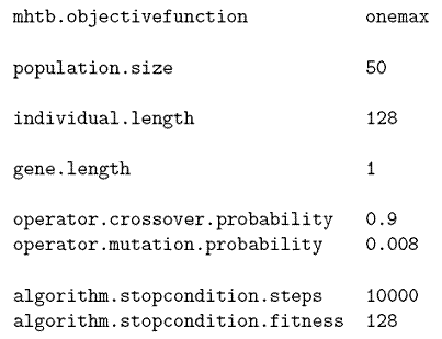
Figure 3: Configuration file for a local execution of the ssGA library.
The first file does not set the mhtb.localeval option, so it takes the default value 2. That is why mhtb.serverlocation, mhtb.serverip, mhtb.serverevalport, mhtb.servercontrolport, mhtb.launchservers and mhtb.delaytime do not make sense. The individuals have a length of 128, the population size is 50, the objective function is onemax and the stop conditions are 10000 iterations or the fitness value of the best individual reaching 128. The crossover probability is 0.9 and the probability of flipping each bit in the mutation process is 0.008.
The algorithm parameters do not change in the second file. But the toolbox general options do. Now there is one instance of the server (mhtb.localeval=0) running in the machine with an IP address of 192.168.3.4, that uses port 5200 to evaluate solutions and port 6200 to receive the stop string. The toolbox will launch and stop the server (mhtb.launchservers=1).
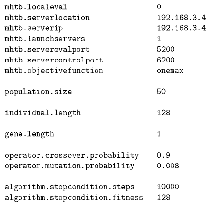
Figure 4: Configuration file for a non-local execution of the ssGA library.
2. jEA
This library admits binary, integer and real representation of the solutions and supports sequential and parallel execution of the algorithms. It offers a large amount of operators. There is also a large number of configuration parameters you may set. We are not enumerating here all the available options but the most relevant ones. We will also present the common options used in all the executions.
| Option | Meaning |
| individual | Kind of individuals representation |
| individual.parameter.length | Individuals length |
| population.size | Population size |
| algorithm.stopcondition | Stop condition |
| result.filename | Results file |
The possible values for individual are GABin (binary individuals), GAInt (integer individuals) and ES (double individuals). The stop condition for the algorithms (algorithm.stopcondition) can be a given number of iterations (SCSteps), the fitness value of the best individual reaching a given value (SCFitness), all the islands finishing their execution in a distributed version of the algorithm (SCDistributed) or some of them combined (SCOr).
To configure the operators of this library you must first indicate the number of them with the operators option. After that, the different options are specified by operator.<i> and operator.<i>.parameter.<param>, where i varies between 0 and operators-1, operator.<i> denotes the name of the operator and param is an operator configuration parameter. The order given by i determines the application order of the operators during the execution of the algorithm. Next, we present some of the operators of this library grouped by categories:
- Selection Operators: These operators pick out individuals from the populaiton and/or the vector of individuals received as a parameter. This library offers a roulette-wheel selection operator (RouletteSelection) with two parameters: select, to determine the number of individuals to be chosen, and include_population, with possible values of yes and no. This parameter determines if the chosen individuals belong to the union of the received vector and the population or only to the received vector, respectively. An operator of selection by tournament is also available (TournamentSelection), with a parameter for setting the tournament size (q), as well as the same two parameters of the previous operator.
- Crossover Operators: Among the available crossover operators we can find the z point crossover (PointCrossover) for binary individuals, with a parameter z to set the number of points to divide the individual into. For integer individuals the partially mapped crossover (PMX), which works with permutations, is available. This operator does not have any parameter. The library also offers a crossover operator for working with Evolutionary Strategies (ESCrossover), which applies uniform crossover to the variables vector and intermediate crossover to the strategic parameters. This operator has two parameters, probability (application probability) and bias (probability of picking each variable from the best parent).
- Mutation Operators: For binary individuals, the bit-flip mutation (BitFlipMu-
tation) is available. It has a probability parameter, which gives the probability of flipping each one of the bits of an individual. The PMutation operator applies to integer individuals representing permutations. It swaps the elements at two chosen randomly different positions with a probability given by probability. For real individuals, the evolutionary strategies mutation operator (ESMutation) is offered. Its application probability is given by probability. - Replacement Operators: This library offers an operator that performs a (μ,λ) replacement (GenerationalReplacement) and another one that performs a (μ+λ) replacement (ElitistReplacement). None of them has parameters.
- Composed Operators: We use them to form more complex operators by combining other ones. All of them contain at least one operator. The composed operator FirstTime contains one operator to be applied only in the first iteration. Its name is set by opname. We have combined this operator with PInitialization to create permutations. Another composed operator is Gap, which applies its contained operator every number of iterations given by gap. It has been combined with Sender to configure the migration of individuals to other subpopulations in distributed executions. The last composed operator we present here is Parallel. It contains one or more operators. It applies all these operators to the received vector of individuals, collects their outputs and returns them concatenated. It has been combined with Dummy, which returns the same vector received as an input, and Receiver, which allows us to receive individuals from other subpopulations.
To illustrate the creation of configuration files for this library we are showing three examples. The first one, Figure 5, corresponds to the solution of the ECC problem with an evolutionary algorithm incorporating a repulsion operator [1] implemented in the library. The second one, Figure 6, allows us to solve the TSP problem. Its interest lies on the use of permutations. Finally, the configuration files to solve the onemax problem in a distributed way (Figures 7, 8 and 9) are shown. They will illustrate the creation of configuration files for parallel executions and the tags system used.
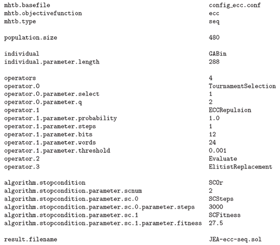
Figure 5: Configuration file to solve the ECC problem with the jEA library.
The first configuration file (Figure 5) configures the library for executing a sequential evolutionary algorithm (mhtb.type=seq) with a population formed by 480 (population.size=480) binary (individual=GABin) individuals with a length of 288 (individual.length=288). To set this library, a file needs to be created. The toolbox will create it and name it config_ecc.conf. The algorithm applies four operators in each iteration. First, a selection by binary tournament (q=2) picks one individual (select=1) from the population. The repulsion operator is applied to this individual with a probability of 1.0. Then, the individual is evaluated (operator.2=Evaluate) and it finally replaces the individual with the worst fitness value in the population (operator.3=ElitistReplacement).
The stop condition is formed by two conditions. The algorithm will end after 3000 iterations or when the fitness value of the best individual reaches 27.5. The results of the execution are stored in a file named JEA-ecc-seq.sol.
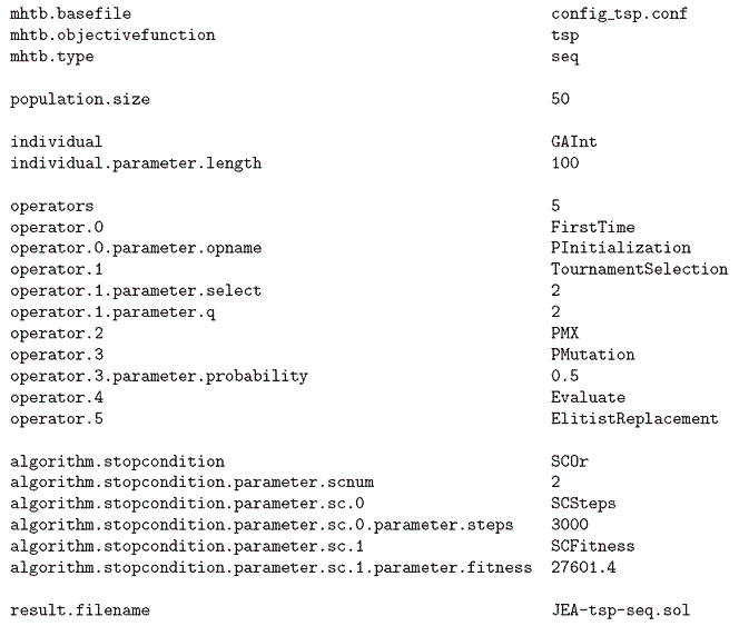
Figure 6: Configuration file to solve the TSP problem with the jEA library.
The configuration file shown in Figure 6 uses integer individuals and it also uses permutation-specific operators. In the first iteration, PInitialization initializes the individuals to contain a valid permutation. In every iteration, two individuals are picked from the population by means of a 2-tournament selection operator, then they are crossed with a permutation-specific operator, the Partially Mapped Crossover (PMX). After that, the two obtained children are mutated with a probability of 0.5. Finally, the individuals are evaluated and inserted into the population with an elitist replacement operator. The algorithm ends after 3000 iterations or when the best fitness reaches 27601.4.
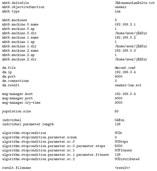
Figure 7: Base file to solve the onemax problem in parallel with the jEA library.
When the jEA library is executed in a distributed way, each one of the islands needs its own configuration file. Most of the content of these files is common to all of them, but certain parameters differ. So, we need to create two configuration files, one with the common parameters and another one with the specific parameters of each island. The first one, see Figure 7, is called base. The operators section is presented in Figure 8. The second file is called delta and its content is shown in Figure 9.
There is a process called DistributionManager, in charge of the synchronization of the parallel execution. To configure it you use a different file, named dm.file in the base file. The base file also contains the machine in which this process will be located (dm.ip), the listening port (dm.port), the incoming connections it will await (dm.connections) and the name of the file to store information about the global execution of the algorithm (dm.result).
The interface of the subalgorithms with this central process is called MessageManager. It is configured by the options msg-manager.host, msg-manager.port and msg-manager.try-time.
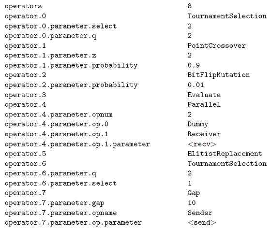
Figure 8: Operators section to solve the onemax problem in parallel with the jEA library.
If you observe the operators section of the base file (Figure 8), you can see the use of the composed operators Parallel and Gap explained above.
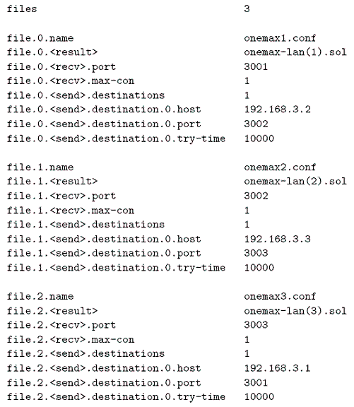
Figure 9: Delta file to solve the onemax problem in parallel with the jEA library.
The configuration options with an specific value for each island are represented by tags in the base file. As an example, the name of the results file is represented by the <result> tag. In the delta file there is one option file.<i>.<result> for each island, which assigns a value to that tag. The same is true for the reception (<recv>) and sending (<send>) of individuals during the migration. The configuration of the sending and reception determines the topology of the subalgorithms. In the example, a unidirectional ring topology is implemented.
The delta file must contain the files option to know how many configuration files need to be created. The value of this parameter must be equal to the value of mhtb.machines.
3. MALLBA
MALLBA is a library of skeletons for combinatorial optimization. The available algorithms are shown in Table 3. This library supports parallel execution and the addition of new operators.
| Skeleton | Description | Solutions encoding |
| newGA | Genetic Algorithm | binary |
| CHC | CHC Algorithm | binary |
| ES | Evolutionary Strategies | real |
| SA | Simulated Annealing | binary |
| CLS | Cooperative Local Search Algorithm | binary |
| newGASA | Hybrid Genetic Algorithm and Simulated Annealing | binary |
This library has a set of general options common to all the algorithms. They are shown in Table 4.
| Option | Values | Meaning |
| algorithm.skeleton | newGA | |
| CHC | ||
| ES | Skeleton we want to use for | |
| SA | solving the problem | |
| CLS | ||
| hybrid | ||
| algorithm.runs | integer > 0 | Number of independent executions |
| algorithm.stopcondition.steps | integer > 0 | Number of iterations per execution |
| algorithm.displaystate | 0-1 | 1: The state is shown on the screen during the execution 0: : It is not shown |
| problem | string | Name identifying the problem to be solved |
| problem.instance | string | Name of the instance file created by the library |
| individual | bin | |
| int | Solutions encoding | |
| float | ||
| individual.length | integer > 0 | Length of the solutions |
| population.size | integer > 0 | Population size (except for SA algorithm) |
| population.offspringsize | integer > 0 | Size of the temporary population created in each iteration (except for SA algorithm) |
| population.replacement | 0-1 | 0: (μ,λ) replacement strategy 1: (μ + λ) replacement strategy |
| result.filename | string | Name of the file to write the execution results into |
The MALLBA library uses a communications library called NetStream, implemented in MPI. For allowing MALLBA to use this library, the value of the conf.mpibindir option needs to be set, so that it contains the path to the /bin directory of the MPICH installation.
The parallel versions of the MALLBA algorithms implement a unidirectional ring topology with a master process that does not explore the search space. This process collects information about the local state of the rest of the processes, and keeps a global state of the parallelized algorithm. To configure these parallel versions we must set the options in Table 5.
| Option | Meaning |
| conf.parallel.globalstate | Number of iterations after which the processes periodically send information about their local state |
| conf.parallel.sync | 0: Asynchronous communication between processes 1: Synchronous communication between processes |
| conf.parallel.checksolutions | Number of iterations after which the processes periodically check the arrival of messages from other processes (except for the SA algorithm) |
| conf.parallel.cooperation | Number of iterations after which the processes periodically cooperate in the search (0: no cooperation) (SA algorithm) |
Next, we show the options for each one of the MALLBA skeletons.
3.1. Genetic Algorithm
This skeleton supports sequential and parallel execution of the algorithm and offers the following operators:
- Selection: The available selection operators are: random selection, selection by tournament, roulette wheel selection, selection by ranking and selection based on the position of an individual in the ordered or reverse-ordered population (rank-based selection). Table 6 shows the configuration parameters offered by the toolbox to set the selection of individuals in this skeleton.
| Option | Values | Meaning |
| operator.selection.parents.id | random tournament roulette ranking best worst |
Random selection Selection by tournament Roulette wheel selection Selection by ranking Rank-based selection (best) Rank-based selection (worst) |
| operator.selection.parents.samplesize | integer > 0 | Size of the sample in the selection b tournament |
| operator.selection.parents.percentage | 1-100 | Skeleton we want to use for |
| operator.selection.parents.position | 0-(pop.size) | Position of the individual in the ordered or reverse-ordered population in the rank-based (best or worst) selection |
- Reproduction: The available reproduction operators for this skeleton are two point
crossover (TPX) and bit-flip mutation. The user can implement his own operators. The
operators option determines the number of operators to be applied in each
iteration of the algorithm (at least one operator). To set the operators, the
options operator.<i> and operator.<i>.<parameter> are needed. The order
assigned by i to the operators will be the order in which these operators will be
applied.
To apply the crossover operator, operator.<i> is set to crossover and operator.
<i>.probability determines the probability of applying it.To apply the mutation operator, operator.<i> is set to mutation; operator.<i>.
applicationprobability determines the probability of applying this operator and operator.<i>.geneprobability the probability of flipping each bit of an individual.If you want to apply a user-implemented operator, operator.<i> must be set to MATLABOperator; operator.<i>.probability determines the probability of applying this operator and operator.<i>.function contains the name of the MATLAB function implementing the operator. The rest of the operator parameters are set in the same way.
If you want to use a different evaluation server, operator.<i>.serverip and operator.<i>.serverport can be set. By default, the same server will be used for evaluation and operators application.
- Replacement: The replacement mechanism used in the population is set by population.replacement. The available methods for choosing the individuals in the next iteration are the same ones used for the selection of parents, and the required parameters to configure them are presented in Table 7.
| Option | Values | Meaning |
| operator.selection.offspring.id | random tournament roulette ranking best worst |
Random selection Selection by tournament Roulette wheel selection Selection by ranking Rank-based selection (best) Rank-based selection (worst) |
| operator.selection.offspring.samplesize | integer >1 | Size of the sample in the selection by tournament |
| operator.selection.offspring.percentage | 1-100 | Percentage of the population used in the selection by ranking |
| operator.selection.offspring.position | 0-(pop.size) | Position of the individual in the ordered or reverse-ordered population in the rank-based (best or worst) selection |
- Migration: When a genetic algorithm is distributed, an operator for exchanging individuals between subpopulations is needed. To configure this migration operator you need to determine the number of individuals to be sent, the selection method to pick them out, the selection method to choose the individuals to be replaced by the new individuals received from other subpopulation and the number of iterations between two migrations. All these operators are shown in Table 8.
| Option | Values | Meaning |
| operator.migration.id | 0 | Migration operator |
| operator.migration.rate | integer | Migration rate |
| operator.migration.individuals | integer | Number of migrated individuals |
| operator.migration.selection.id | random tournament roulette ranking best worst |
Random selection Selection by tournament Roulette wheel selection Selection by ranking Rank-based selection (best) Rank-based selection (worst) |
| operator.migration.selection.samplesize | integer >1 | Size of the sample in the selection by tournament |
| operator.migration.selection.percentage | 1-100 | Percentage of the population used in the selection by ranking |
| operator.migration.selection.position | 0-(pop.size) | Position of the individual in the ordered or reverse-ordered population in the rank-based (best or worst) selection |
3.2. CHC Algorithm
This skeleton supports sequential and parallel execution of the CHC algorithm and it offers the following operators:
- Selection: This algorithm works with all the individuals in the population in the reproductive process. That is why the selection method can not be configured by the user.
- Reproduction: The Half Uniformed Crossover (HUX) operator is available. The user can implement his own operators. The way of setting the reproductive operators is the same seen for the genetic algorithms.
- Replacement: The CHC algorithm implements an elitist replacement. It creates the population of the next iteration by selecting the best individuals from the union of both the population created in the reproductive process and the one in the previous iteration. This replacement operator can not be configured by the user.
- Restart: Due to the quick convergence of this algorithm, when it is detected, a restart operator is applied to partially restart the population. The operator used by this algorithm is a bit-flip mutation operator. operator.diverge.percentage is the percentage of the population to be restarted and operator.diverge.probability is the probability of flipping each bit of a solution.
- Migration: The migration operators are the same ones explained for the genetic algorithms skeleton. They are shown in Table 8.
3.3. Evolutionary Strategies
This skeleton supports sequential and parallel execution and offers the following operators:
- Selection: This skeleton offers the same selection methods as the genetic algorithms skeleton. The configuration parameters for these methods were shown in Figure 6.
- Reproduction: A crossover operator and a mutation operator, specific for the evolutionary strategies, are available. The crossover operator applies uniform crossover to the solution and an intermediate crossover to the strategic parameters (the ones that allow a self-adaptation of the search). The mutation operator also affects both the solution and the strategic parameters. The way of setting these two operators, as well as the user-implemented operators, is the same one seen for the genetic algorithms skeleton, but this mutation operator has only one parameter (applicationprobability).
- Replacement: The replacement is always elitist. So, the replacement operator is not configurable by the user in this skeleton.
- Migration: The configuration parameters for a distributed execution of the algorithm are the same ones given for the previous skeletons. They were presented above in Figure 8.
3.4. Simulated Annealing
This skeleton supports sequential and parallel execution. The implemented cooling schedule is VFSA (Very Fast Simulated Annealing) and the number of iterations between two temperature updates is set by the algorithm.sa.markov-chain parameter.
3.5.Cooperative Local Search
The Cooperative Local Search (CLS) can be seen as a weak hybridization technique. This algorithm works with a population of local solvers. Each one of these solvers performs a local search. They cooperate by exchanging the information obtained during the search. The given implementation of this algorithm uses simulated annealing as the base skeleton.
The specific parameters required by this skeleton are shown in Table 9.
| Option | Meaning |
| algorithm.cls.solvers | Number of solvers |
| algorithm.cls.granularity | Number of steps executed by each solver between cooperations |
| algorithm.cls.base | Base skeleton of the solvers (it must be SA) |
| algorithm.cls.base.runs | Number of independent executions of each solver |
| algorithm.cls.base.stopcondition.steps | Number of iterations in each execution |
| algorithm.cls.base.markov-chain | Number of iterations between temperature updates |
3.6. Hybrid Genetic Algorithm and Simulated Annealing
This skeleton offers three different weak hybridization versions:
- Weak hybridization 1: A simulated annealing algorithm is used as an operator of the genetic algorithm.
- Weak hybridization 2: The genetic algorithm is executed and when it finishes, n solutions are selected from the final population and a simulated annealing algorithm is applied to each one of them. The selection method and the number of selected solutions are chosen by the user.
- Weak hybridization 3: The genetic algorithm is executed and when it finishes, n solutions are randomly selected from the final population with a probability of n∕size(population), and a simulated annealing algorithm is applied to each one of them. The number of selected solutions is determined by the user.
The parameters the user needs to set for this skeleton are shown in Table 10.
| Option | Meaning |
| algorithm.skeleton1 | First skeleton of the hybridization (newGA) |
| algorithm.skeleton2 | Second skeleton of the hybridization (SA) |
| algorithm.hybrid.type | Hybridization version we want to use |
| algorithm.hybrid.passed | Number of solutions passed from the first algorithm to the second one (versions 2 and 3) |
| operator.selection.id | Selection method for the solutions passed from the first algorithm to the second one (version 2) |
| operator.selection.samplesize | Size of the sample in the selection by tournament |
| operator.selection.percentage | Percentage of the population used in the selection by ranking |
| operator.selection.position | Position of the individual in the ordered or reverse-ordered population in the rank-based (best or worst) selection |
The available selection methods are the same ones presented in the previous skeletons. algorithm.hybrid.type accepts the values 1 (weak hybridization 1), 2 (weak hybridization 2) and 3 (weak hybridization 3).
To configure the genetic algorithm, the parameters in Table 11 need to be set.
| Option | Meaning |
| newga.runs | Number of independent executions |
| newga.stopcondition.steps | Number of iterations per execution |
| newga.population.size | Population size |
| newga.population.offspringsize | Size of the temporary population created in each iteration |
| newga.population.replacement | 0: (μ,λ) replacement strategy 1: (μ + λ) replacement strategy |
| newga.displaystate | 1: The state is shown on the screen during the execution 0: It is not shown |
To set the simulated annealing skeleton, the following options are needed: sa.runs (number of independent runs of the algorithm), sa.stopcondition.steps (number of iterations per execution), sa.markov-chain (number of iterations between two temperature updates) and sa.displaystate (1: it shows the state on the screen during the execution, 0: it does not show it).
Once the configuration options for this library have been presented, some examples of configuration files are shown. There is a configuration file to solve the onemax problem with the simulated annealing skeleton (Figure 10). We also show a configuration file to solve the ECC problem with the repulsion operator [1] implemented in MATLAB (Figure 11). Figure 12 shows the lines to be added to the previous file to execute the distributed version of the algorithm on a LAN. Finally, Figure 13 shows the content of a configuration file to solve the onemax problem with the hybrid skeleton.
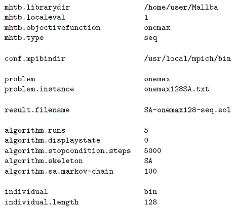
Figure 10: Configuration file for the SA skeleton of MALLBA.
The configuration file for the SA skeleton configures the toolbox for launching an instance of the server in the local machine (mhtb.localeval=1) with 5000 and 6000 as default ports. Five independent runs (algorithm.runs=5) of the sequential (mhtb.type=seq) simulated annealing algorithm are performed, without showing information on the screen during the runs (algorithm.displaystate=0), and updating the temperature every 100 iterations. The solutions encoding is binary (individual=bin), witsh a length of 128. The instance file created by the library will be named onemax128SA.txt and the results will be stored in a file named SA-onemax128-seq.txt.

Figure 11: Configuration file for the newGA skeleton of MALLBA.
The newGA skeleton (Figure 11) performs a single run (algorithm.runs=1) with 3000 iterations (algorithm.stopcondition.steps=3000). As the mhtb.localeval is not set, the process-level evaluation by default is used. The algorithm handles a population of 480 binary individuals, with an individual length of 288 (population.size=480, individual=bin and individual.length=288). One single individual is selected in each iteration (population.offspringsize=1) by a binary tournament (operator.selection.parents.id=tournament and operators.selection.parents.samplesize=2). Only one operator is applied to this solution (operators=1). This operator is implemented in MATLAB (operator.0=MATLABOperator). The function implementing the operator is ecc_repulsion and the application probability of this operator is 1.0, that is, the operator is applied in all the iterations. The last four options of the configuration file set the parameters of the operator.
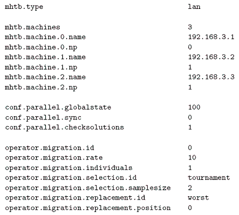
Figure 12: Configuration options for a parallel execution of the newGA skeleton.
Figure 12 shows the lines we need to add/modify in the previous file to run the distributed version of the algorithm. First, you need to change the value of mhtb.type from seq to lan because the execution to be carried out is a parallel one. You also need to set the number of machines to be used (mhtb.machines=3) and the machine to place the master process in (mhtb.machine.0.np=0). Every 10 iterations (operator.migration.rate=10) the migration operator picks out one individual (operator.migration.individuals=1) by a binary tournament and sends it to the next process. After that, the process does not stop awaiting the reception of individuals from other processes (conf.parallel.sync=0). The reception check is performed in all the iterations (conf.parallel.checksolutions=1). When an individual is received, it is inserted into the population, replacing the worst individual in it. The global state of the algorithm is updated every 100 iterations.
You must take into account that the size of the population and the number of iterations appearing in the configuration file for a parallel execution refer to each one of the subpopulations. Therefore, if you want the distributed version of the algorithm to perform the same number of total evaluations (3480), you will set the size of the subpopulations to 160 and the number of iterations to 1000.
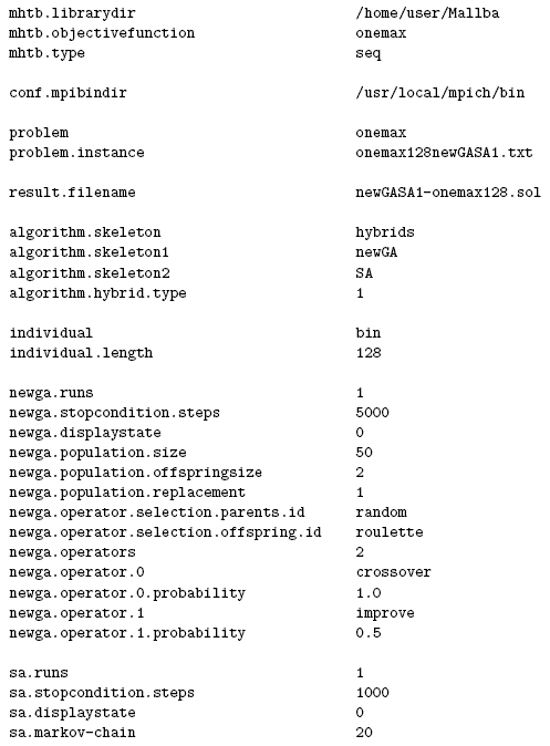
Figure 13: Configuration file for the hybrid skeleton of MALLBA.
The configuration file of the hybrid skeleton (Figure 13) corresponds to a sequential execution with the first version of weak hybridization (algorithm.hybrid.type=1). algorithm.skeleton is set to hybrid and the skeletons taking part in the hybridization are set by algorithm.skeleton1=newGA and algorithm.skeleton2=SA. The simulated annealing algorithm acts as an operator of the genetic algorithm (newga.operator.1=improve). The options of the genetic algorithm have the newga. prefix and the options of the simulated annealing algorithm have the sa. prefix.
If you want to use one of the other two hybridization techniques, you will set the option algorithm.hybrid.type to 2 or 3. You will also establish the number of solutions to apply the simulated annealing to with the algorithm.hybrid.passed option and, if the third hybridization technique is selected (algorithm.hybrid.type=3), you will also set the selection method to pick out these solutions with the options shown in Table 10
